Observaciones influyentes

Correspondiente a la sesión del jueves, 5 de junio de 2025

1. Casos influyentes Multinivel

pacman::p_load(influence.ME,
               lattice, # dotplot
               dplyr,
               texreg,
               stargazer,
               tidyr
                )

Datos (incluidos en el paquete influence.ME)

23 escuelas, 519 individuos
variables principales:
- Dependiente: rendimiento en matemática
- Independiente L1: homework, tiempo realizando tareas
- Independiente L2: structure, grado de estructura de las clases

data(school23)
dim(school23)

str(school23$homework) 
school23 <- within(school23, homework <- unclass(homework)) # pasar a continua
str(school23$homework)

Estimación modelo

m23 <- lmer(math ~ homework + structure + (1 | school.ID),data=school23)

summary(m23, cor=FALSE)

Linear mixed model fit by REML ['lmerMod']
Formula: math ~ homework + structure + (1 | school.ID)
   Data: school23

REML criterion at convergence: 3724.5

Scaled residuals: 
    Min      1Q  Median      3Q     Max 
-2.6617 -0.7063 -0.0151  0.6665  3.2326 

Random effects:
 Groups    Name        Variance Std.Dev.
 school.ID (Intercept) 19.54    4.421   
 Residual              71.31    8.445   
Number of obs: 519, groups:  school.ID, 23

Fixed effects:
            Estimate Std. Error t value
(Intercept)  52.2355     5.3948   9.683
homework      2.3938     0.2771   8.640
structure    -2.0950     1.3239  -1.582

Plot descriptivo

struct <- school23 %>% select(school.ID, structure, math) %>% group_by(school.ID) %>% summarise_all(mean) %>% as.data.frame() 

dotplot(math ~ factor(structure), # lattice
        struct,
        type=c("p","a"),
        xlab="Class structure level",
        ylab="Average Math Test Score")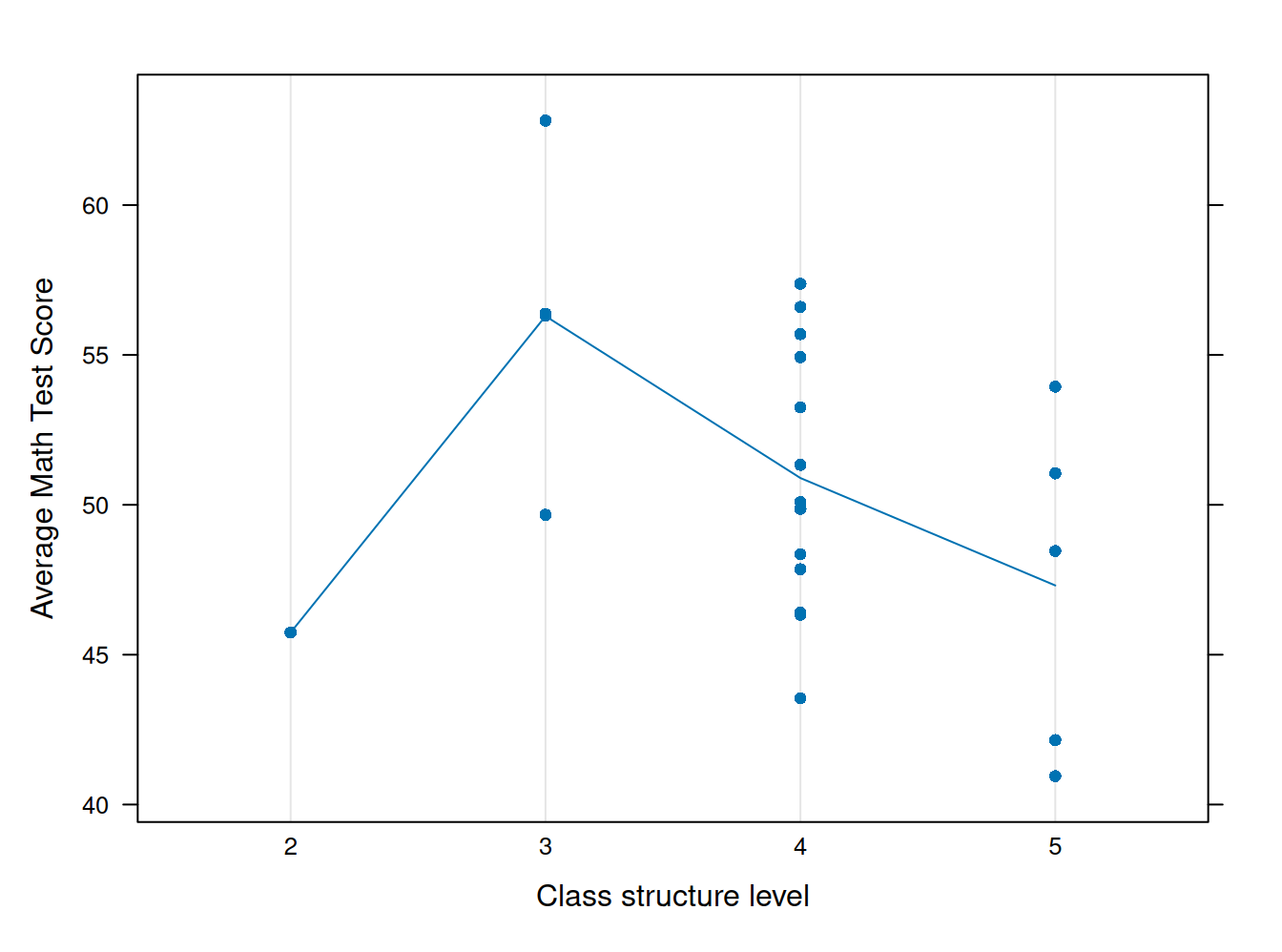

Calculando medidas de influencia basados en función influence de influence.ME

estex.m23 <- influence(m23, "school.ID")

Genera objeto estex.m23 para futuras estimaciones de influencia

DFBETAS

dfbetas(estex.m23)

      (Intercept)    homework    structure
6053   0.20438272 -0.13353782 -0.168112863
6327   0.11706086 -0.44769047  0.020480558
6467  -0.01647348  0.21089491  0.015320693
7194   0.03155659 -0.44641518  0.036749233
7472  -1.20542747 -0.55839049  1.254798224
7474  -0.22112732 -0.51980380  0.353431371
7801   0.07862924 -0.45872039 -0.012145337
7829   0.58739143 -0.77957141 -0.555013123
7930  -0.09131583  0.65291967  0.019638096
24371 -0.07478227  0.37515821 -0.002611182
24725 -0.14550292  0.60660357 -0.005518191
25456  0.07021527 -0.36410988 -0.005086597
25642  0.02256001 -0.21373926 -0.013416556
26537  0.06514836  0.28956822 -0.095167486
46417 -0.01740458  0.26325092  0.023438196
47583 -0.05615965  0.23266306  0.026355535
54344  0.38857969  0.08338389 -0.474978335
62821  0.66202562 -0.92371257 -0.455327896
68448 -0.30385524  0.41369769  0.222734720
68493 -0.05718403  0.25071141 -0.006237296
72080 -0.04604135  0.32986115  0.008072893
72292 -0.11354833  0.62278357  0.003905476
72991 -0.06669580  0.52021276  0.021627589

dfbetas(estex.m23,parameters=c(2,3))

         homework    structure
6053  -0.13353782 -0.168112863
6327  -0.44769047  0.020480558
6467   0.21089491  0.015320693
7194  -0.44641518  0.036749233
7472  -0.55839049  1.254798224
7474  -0.51980380  0.353431371
7801  -0.45872039 -0.012145337
7829  -0.77957141 -0.555013123
7930   0.65291967  0.019638096
24371  0.37515821 -0.002611182
24725  0.60660357 -0.005518191
25456 -0.36410988 -0.005086597
25642 -0.21373926 -0.013416556
26537  0.28956822 -0.095167486
46417  0.26325092  0.023438196
47583  0.23266306  0.026355535
54344  0.08338389 -0.474978335
62821 -0.92371257 -0.455327896
68448  0.41369769  0.222734720
68493  0.25071141 -0.006237296
72080  0.32986115  0.008072893
72292  0.62278357  0.003905476
72991  0.52021276  0.021627589

2/sqrt(23) # cut point

[1] 0.4170288

dfbeta_estex.m32=as.data.frame(dfbetas(estex.m23))

dfbeta_estex.m32 %>%  filter(homework > 0.417 | structure > 0.417 )

      (Intercept)   homework    structure
7472  -1.20542747 -0.5583905  1.254798224
7930  -0.09131583  0.6529197  0.019638096
24725 -0.14550292  0.6066036 -0.005518191
72292 -0.11354833  0.6227836  0.003905476
72991 -0.06669580  0.5202128  0.021627589

plot(estex.m23, which="dfbetas", parameters=c(2,3), xlab="DFbetaS", ylab="School ID")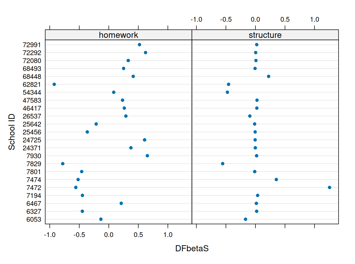

Distancia de Cook

cooks.distance(estex.m23, sort = TRUE)
4/23 # cut point

plot(estex.m23, which="cook",
     cutoff=.17, sort=TRUE,
     xlab="Cooks Distance",
     ylab="School ID")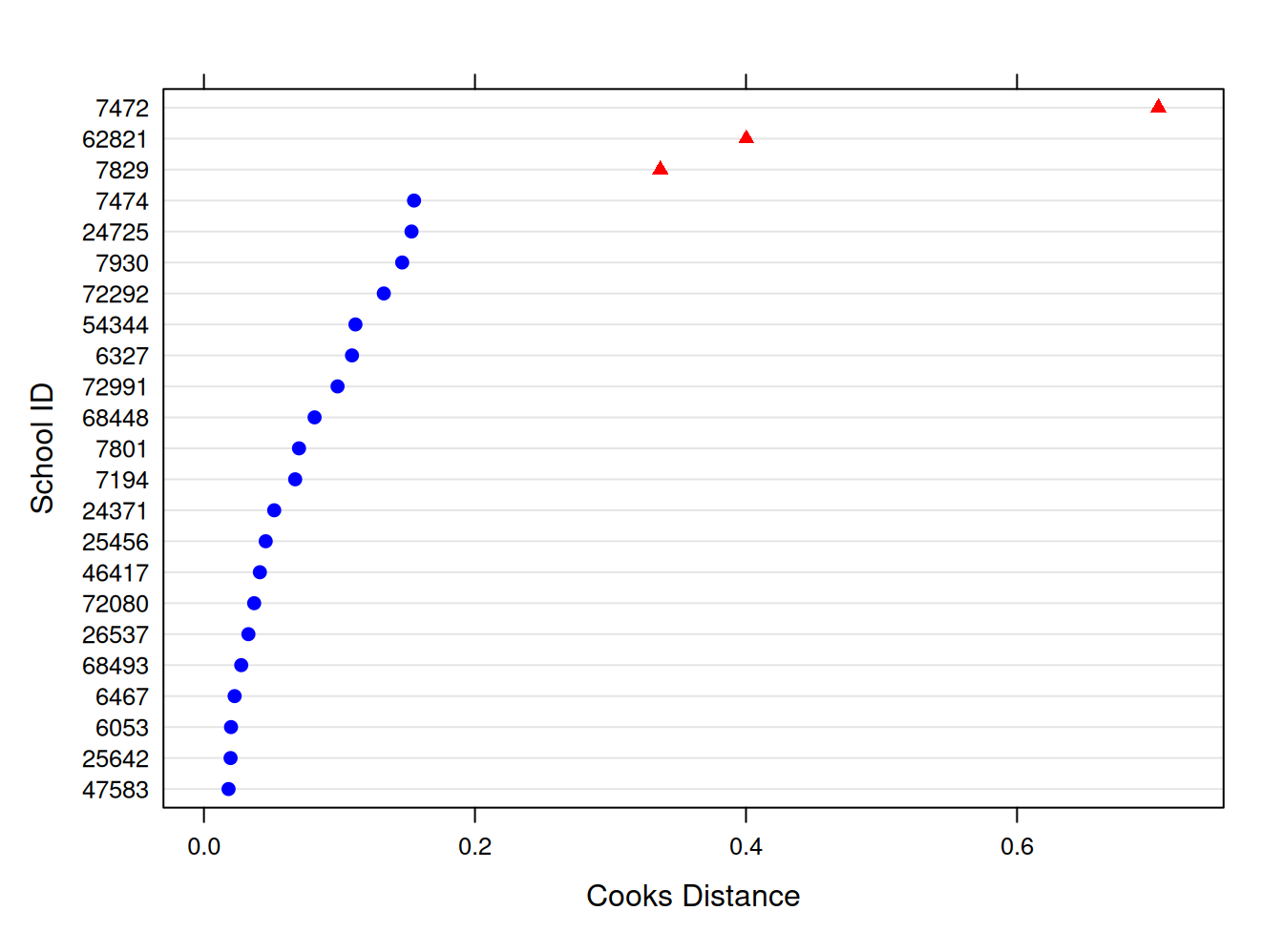

Statistical significance

sigtest(estex.m23, test=-1.96)$structure[1:10,]

      Altered.Teststat Altered.Sig Changed.Sig
6053         -1.326219       FALSE       FALSE
6327         -1.688461       FALSE       FALSE
6467         -1.589753       FALSE       FALSE
7194         -1.512465       FALSE       FALSE
7472         -2.715381        TRUE        TRUE
7474         -1.894861       FALSE       FALSE
7801         -1.533801       FALSE       FALSE
7829         -1.045699       FALSE       FALSE
7930         -1.565893       FALSE       FALSE
24371        -1.546618       FALSE       FALSE

Para la variable structure, se muestran las primeras 10 filas, y se establece un criterio de significación de 1.96 para detectar si hay alteraciones en la significación

datab=filter(school23,school.ID!=7472)

m23b <- lmer(math ~ homework + structure + (1 | school.ID),data=datab)

sjPlot::tab_model(m23, m23b, 
                  show.ci = FALSE,
                  dv.labels = c("Modelo original", "Modelo sin influyentes"))

	Modelo original		Modelo sin influyentes
Predictors	Estimates	p	Estimates	p
(Intercept)	52.24	<0.001	59.41	<0.001
homework	2.39	<0.001	2.55	<0.001
structure	-2.10	0.114	-3.89	0.007
Random Effects
σ²	71.31		70.67
τ₀₀	19.54 _school.ID		15.33 _school.ID
ICC	0.22		0.18
N	23 _school.ID		22 _school.ID
Observations	519		496
Marginal R² / Conditional R²	0.158 / 0.339		0.235 / 0.371

¿Qué diferencia hay entre el modelo con y sin la observación influyente de nivel 2?

1. Casos influyentes Multinivel

Foro